Men nok med en anden tekst. Der er lidt mere relevant. “Trust no one”. Eller måske lidt meta? “Hanlon’s razor”. Så kan folk selv google og gætte. Anyway – det tager lidt tid før jeg bliver færdig med den.

Uncategorized
Hjemmelavet gin
Når man laver sin egen tonic – så bør man vel også lave sin egen gin.
Gin er basalt set en kryddersnaps, hvor den primære smagsgiver er enebær. Det er sådan set definitionen på gin. Så det er jo ikke fordi det er svært.
Jeg er i den lykkelige situation, at jeg fik en Anova precision cooker i fødselsdagsgave sidste år. Og en af de opskrifter der er i den app der knytter an til den, er på sous vide gin.
- Det er helt enkelt:
- 3 ounces (88 ml) vodka
- 10 korianderfrø
- 8 enebær
- 2 stk tørret lavendel
- 5 hele peberkorn
- 2 kardemommekapsler
- 1 laurbær
Det hele smides i en pose der sænkes i vand for at få luften ud, og forsegles. Lynlåsposer anbefales. Dernæst får posen 10 minutter i vandbadet ved 80 grader.
Nu havde jeg ikke korianderfrø i huset. Og det lavendel jeg har, er så findelt at jeg aldrig får siet det fra igen.
Så i stedet lavede jeg en tester:
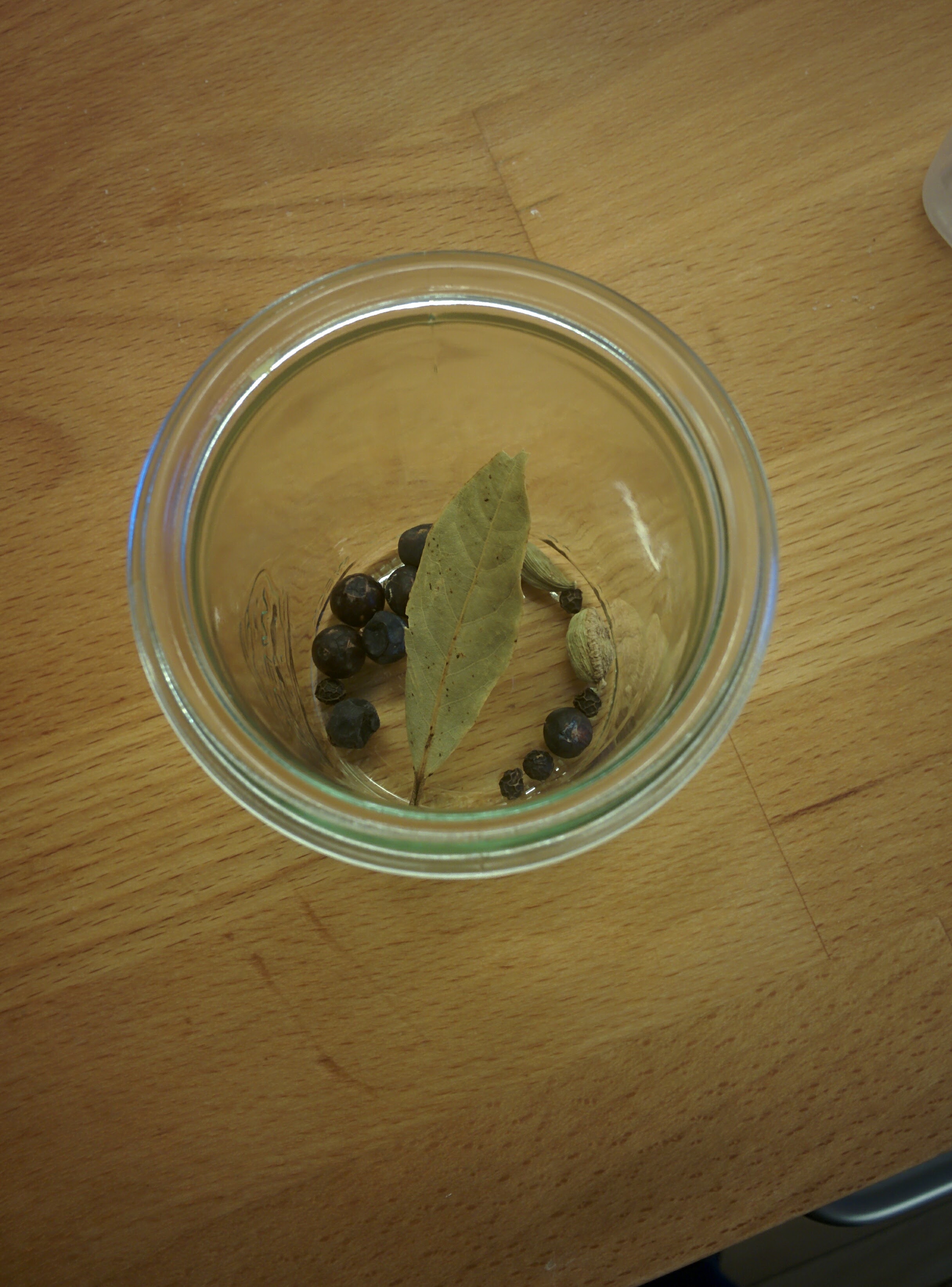
- 90 ml vodka
- 8 enebær
- 1 laurbærblad
- 2 kardemommekapsler
- 5 peberkorn
I stedet for at komme det i en lynlåspose, kom det i et sylteglas (160 ml)
I vandet – 80 grader – 10 minutter. Og så på køl, så jeg ikke skulle prøvesmage varm gin.
Der var ærligt talt ikke så mange nuancer i det – andet end peber, som overdøvede alt andet. Så det var rimeligt givet at der skulle skrues kraftigt ned for den.
Jeg havde annonceret dagens projekt på Facebook – og min lillebror, der også er kreativ i et køkken, kommenterede at han havde prøvet. Og at man med fordel kunne fordoble antallet af enebær. Så der blev lavet ti batches med varierende indhold. Basis i dem alle var:
- 1 laurbærblad
- 2 kardemommekapsler
- 16 enebær
- 3 peberkorn
- 90 ml vodka
Og så variationerne:
Batchnumre, og tilsætning:
 1 allehåndebær
- 2 allehåndebær
- 1 nellike
- 2 nelliker
- 5 fennikelfrø
- 10 fennikelfrø
- 1 lille stjerneanis
- 1 stor stjerneanis
- 5 kommenfrø
- 10 kommenfrø.

Alt på glas, der lukkes og sættes på vandbadet. Et ret stort et af slagsen. Normalt bruger jeg min suppegryde til sousvidingen. Men jeg ville godt lave alle 10 glas på en gang. Jeg kunne selvfølgelig bare lave fem ad gangen. Krydderurterne skal jo filtreres fra, og det kunne jeg passende gøre mens de næste fem kom i gryden. Men bagefter havde jeg planlagt at glassene skulle i brug igen til næste uges morgenmad (man kan ane dele af det på panden i baggrunden). Og der skulle de være i vandet i en time. Og så ville det blive lidt for bøvlet. Så ned i kælderen og finde en termokasse – vi bruger dem når min vi holder fødselsdag for min mand, og hele svigerfamilien + min side er der. Og der derfor skal laves mad til 18 mennesker. Elkedlen op at koge, hælde kogende vand over låget – ja, den kan godt tåle 100 grader. Montere Anovaen, hælde vand i – hold da op hvor skulle der  meget vand i. Så støbejernsgryden og et stort sylteglas kom med ned i kassen. Det endte med at se således ud. Det er strengt taget noget rod at sætte en støbejernsgryde i – den kræver ret meget energi at varme op. Der er jeg nok nødt til at finde en mere fiks løsning til næste gang.
Nå. 80 grader. 10 minutter. Alle glassene blev taget op, og indholdet filtreret over på andre glas. Og så var det sådan set bare at vente på at det var blevet så koldt, at man kunne prøvesmage. Jeg har ikke taget billeder af prøverne – de var stort set ens. Det der er pointen er egentlig, at det ligner urinprøver. Det er meget gult, og det kunne nok være interessant at teste hvor farven egentlig kommer fra. Jeg har – baseret på tidligere eksperimenter med pebersnaps – en fornemmelse af at det i ret høj grad er peberen der giver meget af farven.
Anyway. Hvordan smagte det?
Batch 1 og 2. Det var dem med allehånde. Den bliver ret kraftigt krydret. 2 allehåndebær er klart for meget. Og 1 enkelt er faktisk også i overkanten.
Nellikerne i batch 3 og 4. Nelliken er meget tydelig allerede med en enkelt nellike. Så batch nr. 4 smagte ikke overraskende alt for meget af nellike.
Så var der fenikel. Det smagte klart anderledes end de andre udgaver. 10 fennikelfrø er efter min mening ikke for meget.
Stjerneanis. Batch 7 og 8. Der skal helt klart stjerneanis i den endelige opskrift. Men ikke en hel. Den lille smagte af lidt for meget – det skal være gin, ikke ouzo. Så i hvert fald ikke en hel stor stjerneanis.
Kommen. Nixen bixen. Der var ikke meget stor forskel på batch 9 og 10. Men der skal nok ikke kommen i overhovedet.
Samtlige batches, det der var tilbage efter jeg havde prøvesmagt – blev hældt sammen. Der er stadig lidt over halvdelen tilbage. I virkeligheden er jeg mere til rødvin end gin.
Næste forsøg? Ja, jeg skal have lidt styr på hvor farven kommer fra. Jeg tror meget af det kommer fra peberen. Og når jeg egentlig ikke er så meget til peber, så kan det jo være lige meget.
Så skal jeg have styr på kvantificeringen af stjerneanisen. Det er ikke specielt præcist at angive “lille stjerneanis”. Jeg skal have fundet ud af hvordan jeg får skruet ned for nelliken. og allehånden. Og så skal det naturligvis overvejes hvilke andre smagsgivere jeg kan komme i.
Fake News. And the importance of numbers
Or rather, the importance of all the numbers.
This is not a political blog. On the other hand, I am a firm believer in facts. There is an objective truth out there. And the world can, more or less, be explained by numbers. And when facts and numbers are weaponized in political struggles, well, it’s hard to avoid wandering in to dangerous territory.
And with that disclaimer out of the way. Recently I saw a graphic making the rounds on Facebook. A simple table listing median household income in the US by race. The numbers are said to come from the US Census Bureau.
The idea is to document that “white privilege” does not exist. “See all the people that are not white, who makes more money than whites”.
Could this be true? As a european, my expectation would be, that white, caucasian, americans are in general terms better off than, for lack of a better word, non-whites, in the US (see, this is dangerous territory, what words do I dare to use?).
One of the great things about US federal institutions is that they generally provides quite free access to their data. I did not have the patience to learn how to navigate their website. Someone at Wikipedia did. And have made this nifty table.
I’m not going to copy all the data. There’s a LOT. But there is three tables. Median household income by race, by ancestry, and by native american tribe. Let us take a look at the first:
| Rank | Race | Median household income (2015 USD) |
| 1 | Asian-American | 91,440 |
| 2 | White | 59,698 |
| 3 | Native Hawaiian and other pacific islander | 55,607 |
| 4 | Some other race | 42,461 |
| 5 | American Indian and Alaska Native | 38,530 |
| 6 | Black or African American | 36,544 |
The numbers does not quite match. But “white” at 59,698 USD compares OK with the 60,256 USD in the graphic. The graphic claims that the numbers are from 2014. The Wikipedia numbers are from 2015. Small differences should not throw us off course.
That is more in sync with my expectations. But are the numbers in the table cooked?
Nope. They are actually correct. The next table on Wikipedia lists median household incomes by ancestry. Indian American in the graphic: 101,561 USD. Indian American on Wikipedia: 101,591 USD. Same with Taiwanese. And the others. There is a small detail. The numbers by ancestry appears to come from the 2014 data from the US Census Bureau, and not the 2015. Again, this is a detail. The main point of the graphic is not that Indian Americans make 41,335 USD more than whites, but rather that they make more money. And that Taiwanese Americans do, and that Filipino Americans do and that… well you get the point.
All right, so what is wrong with that table? The thing that is wrong, is that it cherrypicks the data. Let us take a look at the table of median household income by ancestry. Just the first six rows:
| Rank | Ancestry | Income |
| 1 | Indian American | 101,591 |
| 2 | Taiwanese American | 85,566 |
| 3 | Filipino American | 82,389 |
| 4 | Australian American | 81,452 |
| 5 | Israeli American | 79,736 |
| 6 | European American | 77,440 |
I will NOT be dragged into the battles about what constitutes a race, how white you should be to be considered white or the whole topic of trans-racialism.
But in the context of the original table, “European American” is rather white. And when we get to “Danish American” (median income 68,558 USD) we are, statistically speaking, talking about people who are very white.
Conclusion: It is not enough to check that the numbers are correct. You also need to check that you have all the numbers.
Hjemmelavet tonic
I sommers – det vil sige sommeren 2016, var det næsten umuligt at finde et sted hvor man kunne købe kinabark. Det skyldtes, at Politiken havde offentliggjort en artikel, der fortalte hvordan man kunne lave sin egen tonic.
Og så skulle alle hipsterne naturligvis lave deres egen tonic, hvilket var irriterende for mig, for så kunne jeg ikke købe kinabark til at lave min egen tonic. (lad min nu være ærlig, det var ikke noget jeg gjorde før artiklen, jeg fik samme ide som hipsterne).
Men jeg har en god hukommelse, så jeg ventede, og nu er jeg gået igang med at lave min egen tonic. Hipsterne er gået videre til næste mode, og det er igen til at få kinabark.
Jeg startede – det var før jul, med Politikens standardopskrift. Den var OK, men jeg syntes at den smagte for meget af citron(græs). Så nu er jeg gået igang med at udvikle min egen opskrift.
Første forsøg var efter følgende recept:
- 2 stilke citrongræs: 39,3 g
- 6 allehåndebær: 0,4 g
- 1,5 spsk kinabark: 11,3 g
- Citronsyre: 20,0 g
- Stjerneanis: 0,8 g
- Fintrevet skal af 3 økoappelsiner: 16,5 g
- Saften af samme tre appelsiner: 200 ml.
- 1 l vand

Allehånde og stjerneanis knuses let i morteren. Citrongræs klippes i mindre stykker, og knuses i morteren. Alle øvrige ingredienser hældes i en gryde, der bringes i kog.
Fra gryden kom i kog, kogte den under middel varme i 21 minutter under låg.
Hele balladen blev hældt gennem en sigte, og derefter gennem min superbag. Og derefter gennem kaffefiltre. Jeg tror jeg nåede op på 15 kaffefiltre, og var nødt til at tage en tur til Fakta for at købe flere.
Og så var klokken blevet mange. Der var hældt 1,2 l væske i gryden, og nu var der 850 ml tilbage – kaffefiltrene havde taget deres del. Så det blev hældt på en bluecap flaske, og sat på køl til dagen efter.
Der var lidt snask i bunden af flasken da jeg hælde den i gryden dagen derpå. Og det var blot det der var fint nok til at komme gennem kaffefiltrene. Anyway. 751 gram sukker blev opløst under opvarmning, blandingen blev bragt i kog, der blev skummet af, og siruppen blev hældt på skoldede flasker.
Og hvordan smagte det så? Jeg fortyndede 42 ml sirup med 80 ml danskvand (fra sodastreameren). Og kunne godt fortyndes noget mere. 50 ml af det fortyndede blev fortyndet til 100 ml. Og så var den tættere på det ønskede resultat. Helt så meget skal den nu ikke fortyndes, jeg skal lande på en mellemproportional. Og så kunne den i øvrigt godt bruge noget mere citrongræs. Måske skulle en af appelsinerne erstattes med en citron. Det prøver jeg næste gang. Politiken foreslog at man kunne eksperimentere, og det er præcist hvad jeg har i sinde at gøre. Så næste forsøg får ud over citron(græs) også en sjat tørrede hyldeblomster.
Andre tip? Næste gang prøver jeg nok at skumme af inden blandingen hældes gennem kaffefiltrene. Citronsyre kan man købe i supermarkedet. Eller på nemlig.com. Der koster det 347,50 kr kiloet.
Man kan også købe det i Matas. Der koster det 137,50 kr kiloet. Jamen er det ikke farligt? Der er jo en faremærkning på! Jo, det kan give alvorlige øjenirritationer hvis man får det i øjnene. Dr. Oetkers fra supermarkedet giver nøjagtig de samme øjenirritationer. Og når man læser på bøtten fra Matas, står der i øvrigt at citronsyren er af levnedsmiddelkvalitet. Så lad være med at gøre nogen rige på at putte citronsyre i små poser.
Hvor meget får man ud af det? Jeg målte ikke. Men der var nok til at fylde 4 kvartlitersflasker. Og så en sjat til (det var de 42 ml fra tidligere). Jeg skal have set på hvad der egentlig sker af volumenændringer når man opløser sukker i vand.
Bemærk også at jeg har vægtangivelser på her. Politiken angiver et antal stilke citrongræs. Men der er katten til forskel på sådan nogen stilke. De fortæller også at man skal bruge 1½ spsk kinabark. Men hvor meget er det? Vægt angivelser er langt mere præcise og reproducerbare.
Lige hvad kinabarken angår. Der testede jeg faktisk. Jeg tog en spsk (det er i øvrigt 15 ml) kinabark 20 gange, og vejede det. Det gav følgende resultater (alle mål i gram):
| 8,5 | 7,5 | 7,3 | 7,9 | 7,8 |
| 6,5 | 7,4 | 8,1 | 7,7 | 7,6 |
| 6,8 | 7,5 | 7,5 | 7,0 | 6,8 |
| 7,6 | 7,9 | 7,6 | 7,3 | 7,7 |
Se, det er pænt store variationer. Der er tal mellem 6,5 og 8,5 gram. Hvis Politiken brugte det mindste mål, og jeg brugte det største – så er det en forskel på vores opskrifter på 30%. Det er faktisk ret meget.
Så i stedet regnede jeg snittet ud – det er 7,5 g pr 15 milliliter. Eller 0,5 gram/ml. Og når Politiken angiver at man skal bruge 1½ spsk – hvilket så svarer til 22,5 ml, finder man ud af at der bør vejes 11,25 g kinabark af. Så præcis er min vægt ikke, så det blev til 11,3 g.
Stuff to keep in mind
Cynical lessons for lower middle management in times of change.
- There are no one else but you, that takes care of you.
- Do not expect any kind of support. It might come, but don’t count on it.
More lessons to come as I finally learn them.
Skat og selvtægt
Kritikere, jeg selv inklusiv, bruger undertiden ordet “natvægterstat”, når vi skal beskrive hvad det er for et samfund Liberal Alliance ønsker. Det er ikke helt retfærdigt. Men det vi mener er, at LA ønsker at skatten skal sættes så langt ned, at det eneste samfundet, staten, kan levere af serviceydelser er en natvægter. En mand der går rundt i byens gader ved nattetide med en kæp og giver tæsk til misædere. Alt det andet er ligegyldigt.
Når det ikke er helt rimeligt, er det fordi LA jo faktisk vil have andre ting end blot en nattevagt. De vil godt have infrastruktur og andet godt.
Når der er en pointe, er det, fordi natvægteren er det logiske slutpunkt når man vil sænke skatter. Natvægteren er samfundets voldsmonopol. Og voldsmonopolet og skatteopkrævningen hænger tæt sammen.
Voldsmonopolet plejer at blive defineret af Max Weber: “En stat er en realitet, hvis og for så vidt dens embedsvæsen effektivt formår at opretholde monopolet på legitim fysisk tvang”.
Det er en social kontrakt mellem den abstrakte definition vi kalder staten, og de meget konkrete mennesker der indgår i den. Kun staten har lov til at bruge vold. Jeg må ikke hævne mig. Jeg skal gå til staten, som så straffer den person der har gjort mig fortræd. Det er et forbud mod selvtægt. For de islandske sagaer har vist hvor uhensigtsmæssige fejder og hævn er.
Det hænger sammen med den personlige ejendomsret og skatteopkrævningen. Det her er mine penge. Og jeg har indgået en social kontrakt med staten om at kun den, efter nærmere bestemte regler, har lov til at tage dem fra mig med magt. Handelen er, at hvis staten beskytter mig mod at andre tager mine penge så afleverer jeg frivilligt nogen af dem. Uden at staten skal bruge kræfter på at udøve vold mod mig.
Det går langt tilbage. Den danegæld vi opkrævede i England i sin tid var en skat. Opkrævet efter princippet om at hvis ikke de gav os deres sølv, så slog vi dem ihjel. Det næste trin er at statsdannelsen beskytter befolkningen mod at andre opkræver skat, at andre tager vores penge. Staten straffer tyveknægte, fordi den ikke bryder sig om konkurrence.
Og sådan hænger det hele så smukt sammen. Jeg giver frivilligt nogen af mine værdier til staten, der dermed slipper for besværet med at tage dem med magt. Til gengæld beskytter den mig mod tyveknægte og voldsforbrydere. Alt det andet med kontanthjælp, kollektiv trafik og sygehuse er først kommet til for nylig.
Og det er her det bliver farligt, når borgerne i en stat oplever at staten ikke længere kan beskytte dem og deres værdier. Hvis staten ikke beskytter mig mod tyveknægte, så bliver jeg nødt til at gøre det selv. Hvis staten ikke kan beskytte mig mod vold, så bliver jeg nødt til at gøre det selv. Og hvis staten ikke kan finde ud af at udøve vold på mine vegne mod en forbryder, så kan den heller ikke finde ud af at gøre det mod mig. Og så kan jeg endda hævne mig uden at samfundet kommer efter mig.
Det simpelthen grundlaget for statens eksistens, jf. Weber, at den kan beskytte sit monopol på vold.
Så hvad er det der sker når borgerne oplever at politiet kun kommer hvis der er stjålet for mere end 100.000 kr i indbruddet? Hvad sker der, når borgerne oplever, at politiet slet ikke kommer, når borgerne ringer efter hjælp når deres børn bliver overfaldet på gaden?
Der sker ganske enkelt det at grundlaget for at hævde at staten stadig eksisterer, eroderer. Det forsvinder.
Så når vi kalder slutpunktet for Liberal Alliances skattepolitik for “natvægterstaten”, så er det fordi vi fornemmer at de ønsker så lidt stat som overhovedet muligt. Og den minimale stat er en stat, der beskytter skatteyderne mod andres skatteopkrævning. Når tyven stjæler din computer, har han opkrævet skat hos dig. Illegitimt. Og det skal staten beskytte dig mod.
Og hvis staten ikke engang kan det – så ophører den med at eksistere.
https://christianknudsen.info/wp-admin/post.php?post=493&action=edit
Let’s be honest. I am easily distracted. While I was thinking about how to plot networks of coauthorships in Acta Chemica Scandinavica, I tinkered with getting data on my twitter-following.
Thats easy enough, but I thought it would be cool to map them. While googling that (I know. There are automated ways to do that, there are scripts I can just copy. Its not difficult. I just want to do it myself.) I stumbled across some neat heatmaps visualizing the distance to fastfood outlets in the US. That looked like fun.
So now, I’m hammering away at that at the moment….
What to map? I need coordinates. For some reason I thought of 7/11. Probably something with those US fastfood stores. Anyway, http://www.7-eleven.dk/find-butik/ has a map. And coordinates on the page!
Save, download. Delete everything that does not contain coordinates. Keep the parts with “value=[coordinates]”. And save the file. And then, some R. Set the working directory, readlines, use stringfunctions to extract the coordinates:
rm(list=ls())
setwd("~/Desktop/711")
koo <- readLines("711_coordinates.html")
koo_list <- c()
for(i in 1:length(koo)){
  res <- strsplit(koo[i], 'value=\"')
  res <- strsplit(res[[1]][2],'\">')
  res <- res[[1]][1]
  koo_list <- c(koo_list, res)
}
I have a nagging suspision that there are repeated coordinates. Lets get rid of those, and take a look:
koo <- unique(koo_list)
head(koo)
## [1] "55.68096,12.58000" "55.681899,12.583777" "55.68216,12.57454"
## [4] "55.67787,12.58015" "55.68225,12.57044" "55.68284,12.57098"I need to get that into a dataframe:
koo_df <- data.frame(lat=character(), lng=character(), stringsAsFactors=FALSE)

for(i in 1:length(koo)){
  koordinat <- strsplit(koo[i],',')
  new_row <- c(as.numeric(koordinat[[1]][1]),as.numeric(koordinat[[1]][2]))
  koo_df <- rbind(koo_df, new_row, stringsAsFactors=FALSE)

}
colnames(koo_df) <- c("lat", "lng")
tail(koo_df)
## lat lng
## 181 57.05891 9.92778
## 182 57.15559 9.73841
## 183 57.45580 10.04221
## 184 57.45665 9.98596
## 185 57.44108 10.53995
## 186 NA NAOh, and I should get rid of any missing values:
row.has.na <- apply(koo_df, 1, function(x){any(is.na(x))})
koo_df <- koo_df[!row.has.na,]
I need some libraries:
library("maps")
library("mapdata")
library('sp')
library('maptools')
## Checking rgeos availability: FALSE
## Note: when rgeos is not available, polygon geometry computations in maptools depend on gpclib,
## which has a restricted licence. It is disabled by default;
## to enable gpclib, type gpclibPermit()library('spatstat')## Loading required package: nlme## Loading required package: rpart##
## spatstat 1.46-1 (nickname: 'Spoiler Alert')
## For an introduction to spatstat, type 'beginner'##
## Note: spatstat version 1.46-1 is out of date by more than 11 weeks; a newer version should be available.Maps helps drawing maps. Mapdata provides maps for the world. sp gives methods for handling spatial data. Lines and polygons eg. I’m going to need that. Maptools is another bunch of tols for handling maps. Spatstat is a set of tools for handling spatial statistical data. I only really need one of them (I think). But it is the most important.
Lets plot something:
kort <- map('worldHires', 'Denmark', col="white", fill=TRUE, bg=NA,
    xlim=c(8,17), ylim=c(53,58), resolution=0)
Map takes a lot of different arguments. The first two: worldHires tells it that it should look to the worldHires map from mapdata. And that we should look specifically to the part called Denmark. col allows me to choose the color of the map – I’m going with black’n’white here. Fill – should the areas be filled with the color (yes, they should, for reasons I’ll get back to.) bg is the background color, and I can limit the part of the map I want to draw. Maps have coordinates as degrees as their natural units. Longitude 8 to 17, latitude 53 to 58 does nicely. The Faroe Islands are in the map (but for some reason not Greenland), I’m not going to bother with them. And Bornholm is going to be cut out later. Well, Bornholm is going to get cut now:
kort <- map('worldHires', 'Denmark', col="green", fill=TRUE, bg="blue",
    xlim=c(8,13), ylim=c(54,58), resolution=0)
Resolution – there are two settings, 0 and 1. 0 gives the highest resolution.
There are some problems here. Smaller islands have disappered. The resolutions is not fantastic. But all that can be easily solved later. The hard part is the following.
Lets get back to the original map, and take a look:
kort <- map('worldHires', 'Denmark', col="white", fill=TRUE, bg=NA,
    xlim=c(8,13), ylim=c(54,58), resolution=0)
str(kort)## List of 4
## $ x : num [1:11164] 8.66 8.68 8.69 8.7 8.72 ...
## $ y : num [1:11164] 54.9 54.9 54.9 54.9 54.9 ...
## $ range: num [1:4] 8.09 12.62 54.56 57.75
## $ names: chr [1:10] "Denmark" "Denmark:Mors" "Denmark:Mon" "Denmark:Samso" ...
## - attr(*, "class")= chr "map"The kort-variable (kort because that is danish for map) is a list of four lists. x and y that defines the shapes. How that is actually done given that Denmark consist of 1? islands, I have no idea. There is a range. And there are 10 named areas in the object. All of them Denmark, but some of them islands like Mors, Møn etc.
Lets also plot the location of 7/11 stores in Denmark:
map(kort)
points(koo_df$lng, koo_df$lat)
We’ll get back to that.
What I want to plot is a distancemap. Different colors based on how far a given position.
The library spatstat has a methods/function that handles that. It’s called distmap(). It takes an object of class “ppp” – that can be made with the function ppp(), also from spatstat.
ppp() takes two vectors for x and y coordinates, a window, defining the, well, window, of the map. And that is of the class “owinâ€.
Therefore, I should begin by making the point pattern dataset::
A <- ppp(koo_df$lng,koo_df$lat,window=owin(xrange=c(7,13),yrange=c(53,58)))
plot(A)
It looks a bit skewed. But otherwise ok. Distmap() takes the ppp object. So its rather simple to calculate and plot:
z <- distmap(A)

plot(z)
Yeah. Very psychedelic. Looking at it, it appears that the scale is in degrees. The yellow colour should be “2.5”. That more or less matches 2½ degree, if you remember that the y-scale is 5 degrees high.
One can almost see something that looks like the outline of Denmark. It gets easier it you know that it is there.
What would be nice, would be to define a window matching Denmark. Make a cut-out of Denmark in the distancemap.
That can be done. Spatstat has a function as.owin.SpatialPolygons() that can take polygons, defined elsewhere, and convert them to a windows, that can be used in the ppp()-function. It takes an object of the type spatialpolygons. Where do we get that? maptools has a function that can convert a map to spatialpolygons: map2SpatialPolygons(). That function takes a map. And a list of the names saved in that map. We already have those. kort, and kort$names. So, first map2SpatialPolygons:
kort.poly <- map2SpatialPolygons(kort, IDs = kort$names)Then as.owin.SpatialPolygons:
dk.owin <- as.owin.SpatialPolygons(kort.poly)And now I have a nice cutout shapes like Denmark! I can even plot it!!
plot(dk.owin)
Neato! Now I just need to use the dk.owin window when defining the ppp object, rather than the rectangular window I used earlier:
A <- ppp(koo_df$lng,koo_df$lat,window=dk.owin)## Warning in ppp(koo_df$lng, koo_df$lat, window = dk.owin): 20 points were
## rejected as lying outside the specified windowRun the distmap function:
dist <- distmap(A)and plot it:
plot(dist)
Done! I do get a warning. 20 points are outside the window. Not that big a surprise, the map is not very precise. Whole islands are missing! But looking at the original map, and what I get when I plot the window, something is happening. And maybe I should take a closer look at what projection that is being used. After all, Denmark lies on a sphere. And the scale is annoying. I want it in kilometers, not degrees.
Average number of authors in Acta Chem. Scand.
We saw the rapid decline of german as a scientific language in the last installment. But what else can we learn? Given that I do not have access to the full text papers.
Well, what about the number of authors on a given paper?
I have a hypothesis. In the beginning of time, chemistry was a lonely science, where individual scientists worked and published alone.
As the years went by, chemistry became a more collaborative science, with more scientists working together, and also publishing together.
So – the average number of authors on a paper will rise, as a function of time.
There is only one way to see if I’m right. Continue reading “Average number of authors in Acta Chem. Scand.”
Acta network part 1
Lets get to work on the network. I don’t have any citation lists, so what I’m after here, is coauthorship. I’m going to draw on some unpublished work I did on Zika-virus research.
I can begin by disregarding all papers with only one author. I want to keep the publication year – as I want to animate the network.
As always, we’ll begin by reading the data:
data <- readRDS(file="d:\\acta\\consistentdata.rda")
head(data)Animated Acta Chem. Scand.
Okay. I would like to make some networks. I would like to animate them. And I’m quietly harvesting all the pdf’s in order to OCR them, and see what I can learn from that.
Before animating networks, it might be a good idea to animate something simpler.
We went on a visit to my sister in law, and on the rather long trip (by train), I had time to read up on network-graphs in R. Some of the last pages were about animation.
so, without further ado, let me introduce this new library:
library(animation)## Warning: package 'animation' was built under R version 3.2.5I’ll get back to that, lets begin by getting at the data: